Contrastive Flow Matching

Abstract

Unconditional flow-matching trains diffusion models to transport samples from a source distribution to a target distribution by enforcing that the flows between sample pairs are unique. However, in conditional settings (e.g., class-conditioned models), this uniqueness is no longer guaranteed—flows from different conditions may overlap, leading to more ambiguous generations. We introduce Contrastive Flow Matching, an extension to the flow matching objective that explicitly enforces uniqueness across all conditional flows, enhancing condition separation. Our approach adds a contrastive objective that maximizes dissimilarities between predicted flows from arbitrary sample pairs. We validate Contrastive Flow Matching by conducting extensive experiments across varying model architectures on both class-conditioned (ImageNet-1k) and text-to-image (CC3M) benchmarks. Notably, we find that training models with Contrastive Flow Matching (1) improves training speed by a factor of up to $9\times$, (2) requires up to $5\times$ fewer de-noising steps and (3) lowers FID by up to $8.9$ compared to training the same models with flow matching. We release our code at: https://github.com/gstoica27/DeltaFM.git.

1 Introduction

Flow matching for generative modeling trains continuous normalizing flows by regressing ideal probability flow fields between a base (noise) distribution and the data distribution [25]. This approach enables straight-line generative trajectories and has demonstrated competitive image synthesis quality. However, for conditional generation (e.g., class-conditional image generation), vanilla flow matching models often produce outputs that resemble an “average” of the possible images for a given condition, rather than a distinct mode of that condition. In essence, the model may collapse multiple diverse outputs into a single trajectory, yielding samples that lack the expected specificity and diversity for each condition [29, 44]. By contrast, an unconditional flow model—tasked with covering the entire data distribution without any conditioning—implicitly learns more varied flows for different modes of the data. Existing conditional flow matching formulations do not enforce the flows to differ across conditions, which can lead to this averaging effect and suboptimal generation fidelity.

Figure 2: $\Delta$FM yields more discriminative and higher quality trajectories. (left) shows the result of standard flow-matching, where flows are straight but end up overlapping for similar class distributions. (right) shows how the addition of the $\Delta$FM objective results in more distinct flows, resulting in images which are more representative of their respective classes.

To address these limitations and improve generation quality, recent work has explored enhancements to structure the generator’s representations and also proposed inference-time guidance strategies. For example, one approach is to incorporate a REPresentation Alignment (REPA) objective to structure the representations at an intermediate layer with those from a high-quality pretrained vision encoder [44]. By using feature embeddings from a DINO self-supervised vision transformer [5, 31], the generative model’s hidden states are guided toward semantically meaningful directions. This representational alignment provides an additional learning signal that has been shown to improve both training convergence and final image fidelity, albeit at the cost of requiring an external pretrained encoder and an auxiliary loss term. Another popular technique is classifier-free guidance (CFG) for conditional generation [18], which involves jointly training the model in unconditional and conditional modes (often by randomly dropping the condition during training). At inference time, CFG performs two forward passes—one with the conditioning input and one without—and then extrapolates between the two outputs to push the sample closer to the conditional target [29, 18]. While CFG can significantly enhance image detail and adherence to the prompt or class label, it doubles the sampling cost and complicates training by necessitating an implicit unconditional generator alongside the conditional ones [20, 11, 11].

We propose Contrastive Flow Matching ($\Delta$FM), a new approach that augments the flow matching objective with an auxiliary contrastive learning objective. $\Delta$FM encourages more diverse and distinct conditional generations. It applies a contrastive loss on the flow vectors (or representations) of samples within each training batch, encouraging the model to produce dissimilar flows for different conditioning inputs. Intuitively, this loss penalizes the model if two samples with different conditions yield similar flow dynamics, thereby explicitly discouraging the collapse of multiple conditions onto a single “average” generative trajectory. As a result, given a particular condition, the model learns to generate a unique flow through latent space that is characteristic of that condition alone, leading to more varied and condition-specific outputs. Importantly, this contrastive augmentation is complementary to existing methods. It can be applied along with REPA, further ensuring that flows not only align with pretrained features but also remain distinct across conditions. Likewise, it is compatible with classifier-free guidance at sampling time, allowing one to combine its benefits with CFG for even stronger conditional signal amplification.

Inspired by contrastive training objectives, $\Delta$FM applies a pairwise loss term between samples in a training batch: for each positive sample from the batch, we randomly sample a negative counterpart. We then encourage the model to not only learn the flow towards the positive sample but also to learn the flow away from the negative sample. This is achieved by adding a contrastive loss to the flow matching objective, which promotes class separability throughout the flow. Our method is simple to implement and can be easily integrated into existing diffusion models without any additional data and with minimal computational overhead.

We validate the advantages of $\Delta$FM through (1) extensive experiments on conditional image generation using ImageNet images across multiple SiT [29] model scales and training frameworks [29, 44], and (2) text-to-image experiments on the CC3M [37] with the MMDiT [14] architecture. Thanks to contrastive flows, $\Delta$FM consistently outperforms traditional diffusion flow matching in quality and diversity metrics, achieving up to an $8.9$-point reduction in FID-50K on ImageNet, and $5$-point reduction in FID on the whole CC3M validation set. It is also compatible with recent significant improvements in the diffusion objective, such as Representation Alignment (REPA) [44]. By encouraging class separability, $\Delta$FM is able to efficiently reach a given image quality with $5\times$ fewer sampling steps than a baseline Flow Matching model, translating directly to faster generation. It also enhances training efficiency by up to 9$\times$. Finally, $\Delta$FM stacks with classifier-free guidance, lowering FID by 5.7% compared to flow matching models.

2 Related works

Our work lies in the domain of image generative models, primarily diffusion and flow matching models. We augment flow-matching with a contrastive learning objective to provide an alternative solution to classifier free guidance.

Generative modeling has rapidly advanced through two primary paradigms: diffusion-based methods [19, 39] and flow matching [25]. Denoising diffusion models typically rely on stochastic differential equations (SDEs) and score-based learning to iteratively add and remove noise [19]. Denoising diffusion implicit models (DDIMs) [39] reduce this sampling complexity by removing non-determinism in the reverse process, while progressive distillation [34] further accelerates inference by shortening the denoising chain. Advanced ODE solvers [6] and distillation methods [41] have also enhanced sampling efficiency. Despite their success, diffusion models can be slow at inference due to iterative denoising [19].

Flow matching [6] has been designed to reduce inference steps. It directly parameterizes continuous-time transport dynamics for more efficient sampling. Probability flow ODEs [39, 25] learn an explicit transport map between data and latent distributions. Unlike diffusion models, it bypasses separate score estimation and stochastic noise, which reduces function evaluations and tends to improve training convergence [6]. A common type of flow matching algorithm popularized recently is the rectified flow [26], which refines probability flow ODEs through direct optimal transport learning, improving numerical stability and sampling speed. This approach mitigates the high computational burden of diffusion sampling while maintaining high-fidelity image generation with fewer integration steps.

Since both diffusion and flow matching models are trained to match the target distribution of real images, they often produce ‘averaged’ samples that lack the sharp details and strong conditional fidelity [17]. Regardless of how much these models speed up, they often need to be invoked multiple times with unique seed noise to find a high-fidelity sample. In response, guidance techniques have been introduced to substantially promote high-fidelity synthesis. Classifier guidance [12], classifier-free guidance [17], energy guidance [8, 45, 27, 40], and more advanced methods [23, 20, 9, 21, 38] improve fidelity and controllability, without requiring multiple invocations. Although they achieve remarkable performance, they typically still require additional computational overhead. CFG requires calling sampling from a second ‘unconditional’ generation and guiding the ‘conditional’ generation away from the unconditional variant [28, 43, 42, 46]. We adapt the flow matching objective with a contrastive loss between the transport vectors within a batch. By doing so, we achieve the same benefits of CFG, without the additional overhead of needing to train an unconditional generator or using one during inference.

Contrastive learning was originally proposed for face recognition [36], where it was designed to encourage a margin between positive and negative face pairs. In generative adversarial networks (GANs), it has been applied to improve sample quality by structuring latent representations [4]. However, to the best of our knowledge, it has not been explored in the context of visual diffusion or flow matching models. We incorporate this contrastive objective to demonstrate its utility in speeding up training and inference of flow-based generative models.

3 Background and motivation

We focus on flow matching models [25] due to its rising popularity as an effective training paradigm for generative models [24, 1, 2]. In this section, we provide a brief overview of flow matching through the perspective of stochastic interpolants [2, 29], as it pertains to our work.

Preliminaries.

Let $p(x)$ be an arbitrary distribution defined on the reals, and let $\mathcal{N}(0,\mathrm{I})$ be a Gaussian noise distribution. The objective of flow matching is to learn a transport between the two distributions. That is, given an arbitrary $\epsilon\sim\mathcal{N}(0,\mathrm{I})$, a flow matching model gradually transforms $\epsilon$ over time into an $\hat{x}$ that is part of $p(x)$. Stochastic interpolants [2, 29] define this transformation as a time-dependent stochastic process, where transformation steps are summarized as follows,

$$\hat{x}_{t}=\alpha_{t}\hat{x}+\sigma_{t}\epsilon$$ (1)

where $\alpha_{t}$ and $\sigma_{t}$ are decreasing and increasing time-dependent functions respectively defined on $t\in[0,T]$, such that $\alpha_{T}=\sigma_{0}=1$ and $\alpha_{0}=\sigma_{T}=0$. While theoretically, $\alpha_{t},\sigma_{t}$ need not be linear, linear complexity is often sufficient to obtain strong diffusion models [29, 25, 44].

Flow matching.

Given such a process, flow matching models learn to transport between noise to $p(x)$ by estimating a velocity field over an probability flow ordinary differential equation (PF ODE), $dx_{t}=v(x_{t},t)dt$, whose distribution at time $t$ is the marginal $p_{t}(x)$. This velocity is given by the expectations of $\hat{x}$ and $\epsilon$ conditioned on $x_{t}$,

$$v(x_{t},t)=\dot{\alpha}_{t}\mathbb{E}[\hat{x}|x_{t}=x]+\dot{\sigma}_{t}\mathbb{E}[\epsilon|x_{t}=x],$$ (2)

where $\dot{\alpha}_{t},\dot{\sigma}_{t}$ are the time-based derivatives of $\alpha_{t}$ and $\sigma_{t}$ respectively. Since, $\hat{x}$ and $\epsilon$ are arbitrary samples from their respective distributions, $v(x_{t},t)$ is expected “direction” of all transport paths between noise and $p(x)$ that pass through $x_{t}$ at $t$. While the optimal $v(x_{t},t)$ is intractable, it can be approximated with a flow-model $v_{\theta}(x_{t},t)$, by minimizing the training objective:

$$\mathcal{L}^{(FM)}(\theta)=\mathbb{E}\left[||v_{\theta}(x_{t},t)-(\dot{\alpha}_{t}\hat{x}+\dot{\sigma}_{t}\epsilon)||^{2}\right]$$ (3)

Key to understanding the properties of flow matching is the concept of flow uniqueness [25]. That is, flows following the well-defined ODE cannot intersect at any time $t\in[0,T)$. As such, flow models can iteratively refine unique-discriminative features relevant to any $x\sim p(x)$ in each $x_{t}$, leading to more efficient and accurate diffusion paths compared to other training paradigms [25].

Conditional flow matching.

Commonly, $p(x)$ may be a marginal distribution over several class-conditional distributions (e.g., the classes of ImageNet [33]). Training models in such cases is nearly identical to standard flow-matching, except that flows are further conditioned on the target distribution class:

$$\mathcal{L}^{(FM)}_{cond}(\theta)=\mathbb{E}\left[||v_{\theta}(x_{t},t,y)-(\dot{\alpha}_{t}\hat{x}+\dot{\sigma}_{t}\epsilon)||^{2}\right],$$ (4)

where $\hat{x}\sim p(x|y)$. Resultant models have the desirable trait of being more controllable: their generated outputs can be tailored to their respective input conditions. However, this comes at the notable cost of flow-uniqueness. Specifically these models only generate unique flows compared to others within the same class-condition, not necessarily across classes. This inhibits $x_{t}$’s from storing important class-specific features and leads to poorer quality generations. Second, the conditional flow matching objective trains models without knowledge of the distributional spread from other class-conditions, leading to flows that may generate ambiguous outputs when conditional distributions overlap . This increases the likelihood of ambiguous generations that form a mixture between different conditions, restricting model capabilities. We study these effects in Section 5.

4 Contrastive Flow-Matching

We introduce Contrastive Flow Matching ($\Delta$FM), a novel approach designed to address the challenges of learning efficient class-distinct flow representations in conditional generative models. Standard conditional flow matching (FM) models tend to produce flow trajectories that align across different samples, leading to reduced class separability. $\Delta$FM extends the FM objective by incorporating a contrastive regularization term, which explicitly discourages alignment between the learned flow trajectories of distinct samples.

Ingredients.

Let $\tilde{x}\sim p(x|\tilde{y})$ denote a sample drawn from the data distribution conditioned on an arbitrary class $\tilde{y}$, and let $\tilde{\epsilon}\sim\mathcal{N}(0,I)$ represent an independent noise sample. To ensure that the contrastive objective captures distinct flow trajectories, we impose the conditions $\tilde{x}\neq\hat{x}$ and $\tilde{\epsilon}\neq\epsilon$, where $\tilde{y}$ may or may not be equal to $y$. Importantly, we do not assume the existence of a time step $t\in[0,T]$ such that $x_{t}=\alpha_{t}\tilde{x}+\sigma_{t}\tilde{\epsilon}$. Consequently, $\tilde{x}$ and $\tilde{\epsilon}$ represent truly independent flow trajectories in comparison to $\hat{x}$ and $\epsilon$.

The contrastive regularization.

Given $v_{\theta}(x_{t},t,y)$ and an arbitrary $\tilde{x},\tilde{\epsilon}$ sample pair, the contrastive objective aims to maximize the dissimilarity between the estimated flow of $v_{\theta}(x_{t},t,y)$ from $\epsilon$ to $\hat{x}$, and the independent flow produced by $\tilde{x},\tilde{\epsilon}$. We achieve this by maximizing the quantity,

$$E\left[||v_{\theta}(x_{t},t,y)-(\dot{\alpha}_{t}\tilde{x}+\dot{\sigma}_{t}\tilde{\epsilon})||^{2}\right].$$ (5)

Since $\tilde{x}$ is drawn from the marginal $p(x)$ rather than $p(x|y)$, Equation 5 trains flow matching models to produce flows that are unconditionally unique.

Putting it all together.

We now define contrastive flow matching as follows,

$$\begin{split}\mathcal{L}^{(\textsc{$\Delta$FM})}(\theta)=\mathrm{E}\left[\begin{aligned} &||v_{\theta}(x_{t},t,y)-(\dot{\alpha}_{t}\hat{x}+\dot{\sigma}_{t}\epsilon)||^{2}\\ &-\lambda||v_{\theta}(x_{t},t,y)-(\dot{\alpha}_{t}\tilde{x}+\dot{\sigma}_{t}\tilde{\epsilon})||^{2}\end{aligned}\right]\end{split}$$ (6)

where $\lambda\in[0,1)$ is a fixed hyperparameter that controls the strength of the contrastive regularization. Thus, $\Delta$FM simultaneously encourages flow matching models to estimate effective transports from noise to corresponding class-conditional distributions (the flow matching objective), while enforcing each to be discriminative across classes (contrastive regularization). Note that $\Delta$FM can be thought of as a generalization of flow matching, as $\Delta$FM reduces to FM when $\lambda=0$. We study the effects of varying $\lambda$ in Section 5.5.

Implementation.

Contrastive flow matching ($\Delta$FM) is easily integrated into any flow matching training loop, with minimal overhead. Algorithm 1 illustrates the implementation of an arbitrary batch step, where navy text marks additions to the standard flow matching objective. Thus, $\Delta$FM solely depends on the information already available to the flow matching objective at each batch step, without computing any additional forward steps. Furthermore, $\Delta$FM seamlessly folds into flow matching training regimes, making it a “plug-and-play” objective for existing setups.

Algorithm 1 Contrastive Flow-Matching Batch Step

1:Input: A model $v_{\theta}$, batch of $N$ flow examples $F=\{(x_{1},y_{1},\epsilon_{1}),\ldots,(x_{N},y_{N},\epsilon_{N})\}$ where $(x_{i},y_{i})\sim p(x,y)$ and $\epsilon_{i}\sim\mathcal{N}(0,\mathrm{I})$, $\beta$ learning rate, $\lambda=0.05$.

2:Output: Updated model parameters $\theta$

3:$L(\theta)=0$

4:for $i$ in range($N$) do

5:     $t\sim U(0,1),x_{t}=\alpha_{t}x_{i}+\sigma_{t}\epsilon_{i}$

6:     sample $(\tilde{x},\tilde{y},\tilde{\epsilon})\sim F,\text{ s.t. }(\tilde{x},\tilde{y},\tilde{\epsilon})\neq(x_{i},y_{i},\epsilon_{i})$

7:     $\hat{v}=v(x_{t},t,y_{i}),v=\dot{\alpha}_{t}x_{i}+\dot{\sigma}_{t}\epsilon,{\color[rgb]{0.0,0.0,0.5}\definecolor[named]{pgfstrokecolor}{rgb}{0.0,0.0,0.5}\tilde{v}=\dot{\alpha}_{t}\tilde{x}+\dot{\sigma}_{t}\tilde{\epsilon}}$

8:     $L(\theta)+=||\hat{v}-v||^{2}-{\color[rgb]{0.0,0.0,0.5}\definecolor[named]{pgfstrokecolor}{rgb}{0.0,0.0,0.5}\lambda||\hat{v}-\tilde{v}||^{2}}$

9:end for

10:$\theta\leftarrow\theta-\frac{\beta}{N}\nabla_{\theta}L(\theta)$

Figure 3: Contrastive Flow-Matching intrinsically separates flows between classes. We train a small three layer MLP flow-matching model to transport between a two dimensional multivariate noise distribution (violet) and two independent blue and orange class distributions respectively. The class distributions are designed to have $\sim 50\%$ overlap, and we plot the learned class-conditioned flows between noise samples and each respective class distribution using class colors. Top: Flow-matching models learn overlapping transports between distributions, generating outputs that lie in ambiguous regions between the two classes. Bottom: Contrastive flow-matching models have significantly more discriminative flows, generating class-coherent samples while reducing ambiguity.

Discussion.

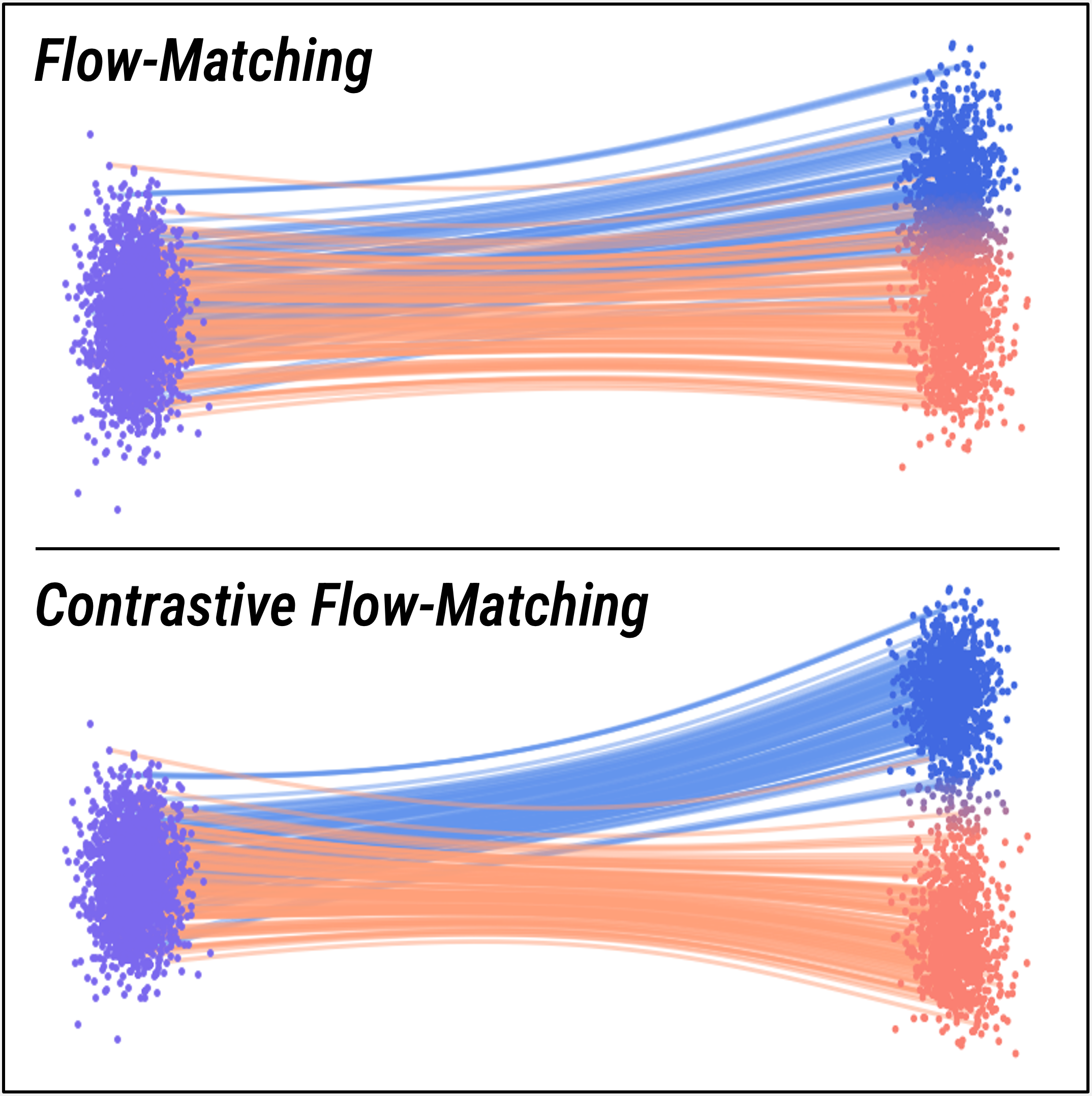
Figure 3 illustrates the effects of contrastive flow matching compared to flow matching. The figure shows the resultant flows after training a small diffusion model in a simple toy-setting. Specifically, we create a two-dimensional violet gaussian noise distribution and two independent two-dimensional class distributions (in blue and orange respectively) such that the latter distributions have $\approx 50\%$ overlap. Samples from each distribution are represented as “dots”, with those in the target distributions colored according to the gaussian kernel-density estimate between samples from each class in their respective region. We observe that training the model with flow matching (top) create flows with large degrees of overlap between classes, generating samples with lower class-distinction. In contrast, training the same model with contrastive flow matching (bottom) yields trajectories that are significantly more diverse across classes, while also generating samples which capture distinct features of each respective class.

5 Experiments

We validate contrastive flow-matching ($\Delta$FM) through extensive experiments across various model, training and benchmark configurations. Overall, models trained with $\Delta$FM consistently outperform flow-matching (FM) models across all settings.

Datasets.

We conduct both class-conditioned and text-to-image experiments. We use ImageNet-1k [10] processed at both ($256\times 256$) and ($512\times 512$) resolutions for our class-conditioned experiments, and follow the data preprocessing procedure of ADM [12] We then follow [44] and encode each image using the Stable Diffusion VAE [32] into a tensor $z\in\mathbb{R}^{32\times 32\times 4}$. For text-to-image (t2i), we use the Conceptual Captions 3M (CC3M) dataset [37] processed at ($256\times 256$) resolution and follow the data processing procedure of [3]. We train all models by strictly following the setup in [44], and use a batch size of 256 unless otherwise specified. We do not alter the training conditions to be favorable to $\Delta$FM, and we always set $\lambda=0.05$ when applicable.

Measurements.

We report five quantitative metrics throughout our experiments. We report Fréchet inception distance (FID) [16], inception score (IS) [35], sFID [30], precision (Prec.) and recall (Rec.) [22] using 50,000 samples for our class-conditioned experiments. Similarly, we report FID over the whole validation set in the text-to-image setting. We use the SDE Euler-Maruyama sampler with $w_{t}=\sigma_{t}$ for all experiments, and set the number of function evaluations (NFE) to 50 unless otherwise specified.

5.1 Contrastive Flow-Matching Improves SiT

Implementation details.

We train on the state-of-the-art SiT [29] model architecture, using both SiT-B/2 and SiT-XL/2.

	Metrics
Model	FID $\downarrow$	IS $\uparrow$	sFID $\downarrow$	Prec. $\uparrow$	Rec. $\uparrow$
SiT-B/2	42.28	38.04	11.35	0.5	0.62
+ Using $\Delta$FM	33.39	43.44	05.67	0.53	0.63
SiT-XL/2	20.01	74.15	8.45	0.63	0.63
+ Using $\Delta$FM	16.32	78.07	5.08	0.66	0.63

(a) ImageNet-1k (256x256) Results. $\Delta$FM significantly outperforms flow-matching models across nearly all metrics, and matches Recall on SiT-XL/2.

	Metrics
Model	FID$\downarrow$	IS$\uparrow$	sFID$\downarrow$	Prec.$\uparrow$	Rec.$\uparrow$
SiT-B/2	50.26	33.58	14.88	0.57	0.61
+ Using $\Delta$FM	41.59	38.20	06.13	0.62	0.63
SiT-XL/2	22.98	70.14	10.71	0.73	0.60
+ Using $\Delta$FM	19.67	72.58	04.98	0.76	0.60

(b) ImageNet-1k (512x512) Results. Models trained with $\Delta$FM either substantially outperform or match their flow-matching counterparts in all metrics.

Table 1: SiT [29] results on ImageNet-1k ($256\times 256$; a) and ($512\times 512$; b). We train all models for 400K iterations following [44]. All metrics are measured with the SDE Euler-Maruyama sampler with NFE=50 and without classifier guidance. We use $\lambda=0.05$ for all models trained with $\Delta$FM and do not change any other hyperparameters. $\uparrow$ indicates that higher values are better, with $\downarrow$ denoting the opposite.

Results.

Table 1 summarizes our results. Overall, $\Delta$FM dramatically improves over flow-matching in nearly all metrics (only matching the flow-matching SiT-XL/2 model in recall). Notably, employing $\Delta$FM with SiT-B/2 lowers FID by over 8 compared to flow-matching at both ImageNet resolutions, highlighting the strength of $\Delta$FM in smaller model scales. Similarly, $\Delta$FM is robust to larger model scales and outperforms FM by over 3.2 FID when using SiT-XL/2.

5.2 REPA is complementary

REPresentation Alignment (REPA) [44] is a recently introduced training framework that rapidly improves diffusion model performance by strengthening its intermediate representations. Specifically, REPA distills the encodings of foundation vision encoders (e.g., DiNOv2 [5]) into the hidden states of diffusion models through the use of an auxilliary objective. Notably, REPA can improve the training speed of vanilla SiT models by over $17.5\times$, while further improving their performances [44]. $\Delta$FM is easily integrated into REPA and only requires replacing the flow-matching objective.

Implementation details.

We apply REPA on the same SiT models as in Section 5.1, and use the distillation process defined by [44] exactly. Specifically, we use distill DiNOv2 [5] ViT-B [13] features into the 4th layer of the SiT-B/2, and the 8th layer of the SiT-XL/2, and mirror their hyperparameter setup.

	Metrics
Model	FID $\downarrow$	IS $\uparrow$	sFID $\downarrow$	Prec. $\uparrow$	Rec. $\uparrow$
REPA SiT-B/2	27.33	061.60	11.70	0.57	0.64
+ Using $\Delta$FM	20.52	069.71	05.47	0.61	0.63
REPA SiT-XL/2	11.14	115.83	08.25	0.67	0.65
+ Using $\Delta$FM	7.29	129.89	04.93	0.71	0.64

(a) ImageNet-1k (256x256) Results with REPA. Adding $\Delta$FM to REPA further improves SiT models across nearly all metrics, and by as much as 6.81 FID.

	Metrics
Model	FID$\downarrow$	IS$\uparrow$	sFID$\downarrow$	Prec.$\uparrow$	Rec.$\uparrow$
REPA SiT-B/2	31.90	056.96	13.78	0.67	0.62
+ Using $\Delta$FM	24.48	064.74	05.89	0.71	0.61
REPA SiT-XL/2	11.32	119.72	10.21	0.76	0.63
+ Using $\Delta$FM	7.64	131.50	04.72	0.79	0.62

(b) ImageNet-1k (512x512) Results with REPA. $\Delta$FM is robust with REPA at large image resolutions, further improving performance across established metrics.

Table 2: REPA SiT [29] results on ImageNet-1k ($256\times 256$; a) and ($512\times 512$; b). All models are trained for 400K iterations strictly following the procedure in [44], and set $\lambda=0.05$. We use the SDE Euler-Maruyama sampler with NFE=50 without classifier guidance for all our metrics.

Results.

We report results in Table 2. Similar to Section 5.1, $\Delta$FM substantially improves REPA models by as much as 6.81 FID, and consistently improves flow-matching with model scale. This highlights the versatility of the contrastive flow-matching objective as a broadly applicable criterion for diffusion model.

Figure 4: Contrastive flow-matching ($\Delta$FM) denoises significantly more efficiently than flow-matching. We visualize the expected final image estimated by a flow-model when denoised every 5 steps for trajectories of length 30 steps using the SDE Euler-Maruyama sampler and do not use classifier guidance. We compare the trajectories of a REPA SiT-XL/2 [44] trained on ImageNet-256 [10] for 400K steps with flow-matching (FM), and the same model trained with the contrastive flow-matching ($\Delta$FM) objective. We show these trajectories in sets of pairs generated from the same noise sample during inference, with the flow-matching model above our $\Delta$FM version.

5.3 Extending to text-to-image generation

Implementation Details.

We train models with the popular MMDiT [14] architecture from scratch on the CC3M dataset [37] for 400K iterations. For faster training, we pair each model with REPA, and follow the recommended training protocol of [44].

Metric	REPA-MMDiT
	Flow-Matching	$\Delta$FM
FID$\downarrow$	24	19

Table 3: $\Delta$FM improves on CC3M 256$\times$256. We use the SDE Euler-Maruyama sampler with NFE=50 without classifier-free guidance.

Results.

Table 3 shows our results. $\Delta$FM improves over the flow matching baseline by $5$ FID, highlighting its seamless transferability to the broader text-to-image setting. We show qualitative results in Appendix A.

5.4 CFG stacks with contrastive flow matching

Contrastive flow matching offers advantages of Classifier-Free Guidance (CFG), without incurring additional computational costs during inference. In this section, we demonstrate that when computational resources permit, combining $\Delta$FM with CFG can yield further performance enhancements.

Accounting for conflicts.

CFG and $\Delta$FM encourage flow matching model generations to be unique and identifiable, in different ways. Specifically, $\Delta$FM trains models whose conditional flows are steered away from other arbitrary flows in the training data, regardless of generation state ($x_{t}$). In contrast, CFG steers generations away from the unconditional flow estimates based on $x_{t}$. Thus, the signals from each may not always be aligned and naively coupling them may lead to conflicts and suboptimal generations. Fortunately, we can quantify the amount of steerage $\Delta$FM applies on flow matching models by deriving the closed-form solution to Eq. 4: $\min_{\theta}\mathcal{L}^{(\Delta\text{FM})}(\theta)=\nicefrac{{\left[(\min_{\theta}\mathcal{L}^{(\text{FM})}(\theta))-\lambda\hat{T}\right]}}{{\left[1-\lambda\right]}}$, where $\hat{T}$ is simply the mean of all sample trajectories from the training set (please see App. B.1 for the full derivation). Thus, $\Delta$FM yields models which estimate flows away from the data-driven unconditional trajectory, weighted by $\lambda$. While optimizer and training dynamics cannot guarantee that all models trained with $\Delta$FM exactly decompose into these terms, $\hat{T}$ nevertheless approximates its effect on these models. With $\hat{T}$, we can account for conflicts between $\Delta$FM and CFG by modifying the CFG equation to: $\hat{\text{CFG}}=(1-\lambda)\left[wv(x_{t}|y)+(1-w)v(x_{t}|\emptyset)\right]+\lambda\tau$, where $w$ is the guidance scale, $\emptyset$ is the unconditional term and $\lambda$ is the same parameter used during $\Delta$FM training (Appendix B.2 contains the full derivation). Note that, we only apply $\hat{\text{CFG}}$ within the specified guidance interval $[\sigma_{\text{low}},\sigma_{\text{high}}]$, and use our unchanged $\Delta$FM model outside this interval.

Model	CFG Terms			Metric
	$w$	$\sigma_{\text{low}}$	$\sigma_{\text{high}}$	IS$\uparrow$	FID$\downarrow$	sFID$\downarrow$
REPA SiT-XL/2	1.75	0.0	0.75	280.33	2.09	5.55
+ Using $\Delta$FM	1.85	0.0	0.65	281.95	1.97	4.49

Table 4: ImageNet 256$\times$256 Results with CFG and NFE=50. “$w$” denotes the classifier-free guidance (CFG) weight, and $[\sigma_{\text{low}},\sigma_{\text{high}}]$ is the time interval under which CFG is applied. We report the best results for each model after conducting a grid search over $w\in\{1.25,1.75,1.8,1.85,2.25\}$, $\sigma_{\text{low}}=0$ and $\sigma_{\text{high}}\in\{0.50,0.65,0.75,1.0\}$. $\Delta$FM outperforms FM on all metrics.

Results.

Table 4 summarizes the results. When paired with CFG, $\Delta$FM improves flow matching models across all metrics, demonstrating its efficacy in settings where computational costs are not a constraint.

Additional Couplings.

While we find that our proposed coupling strategy for $\Delta$FM and CFG works well for our setting, other suitable variations may also exist. For instance, one may instead reduce conflicts by following the equation: $\tilde{CFG}=(w+\lambda)v(x_{t}|y)-(1-w)v(x_{t}|\emptyset)-\lambda\hat{T}$, where $\lambda\text{, and }w$ are free hyperparameters. We leave such exploration to future work.

5.5 Analyzing Contrastive Flow-Matching

Understanding the $\Delta$FM weight ($\lambda$).

$\lambda$ directly controls how unique flows are across classes. Increasing $\lambda$ encourages every diffusion step to be fully discriminative, enabling models to encode distinct representations that integral to generating strong visual outputs at each trajectory step. However, setting it too high can lead to overly-separated flow trajectories, making it difficult to capture the class structure (Table 5). However, $\lambda$ values that are too low mirror the flow matching objective. Notably, we find that $\lambda=0.05$ is stable across all model and dataset settings, consistently achieving strong performance.

Metric	$\Delta$FM $\lambda$ Values
	$0.0$	$0.001$	$0.01$	$0.05$	$0.1$	$0.15$
IS$\uparrow$	115.83	115.70	119.41	129.89	116.27	82.20
FID$\downarrow$	11.14	10.93	9.93	7.29	9.86	19.21

Table 5: $\lambda=0.05$ is ideal. We show an ablation of the $\Delta$FM weight parameter $\lambda$. A too large $\lambda$ produces degenerate distributions that do not model class structure well. Too low $\lambda$ is essentially identical to flow-matching, with very little effect on training. $\lambda=0.05$ is best and we use this for all our experiments.

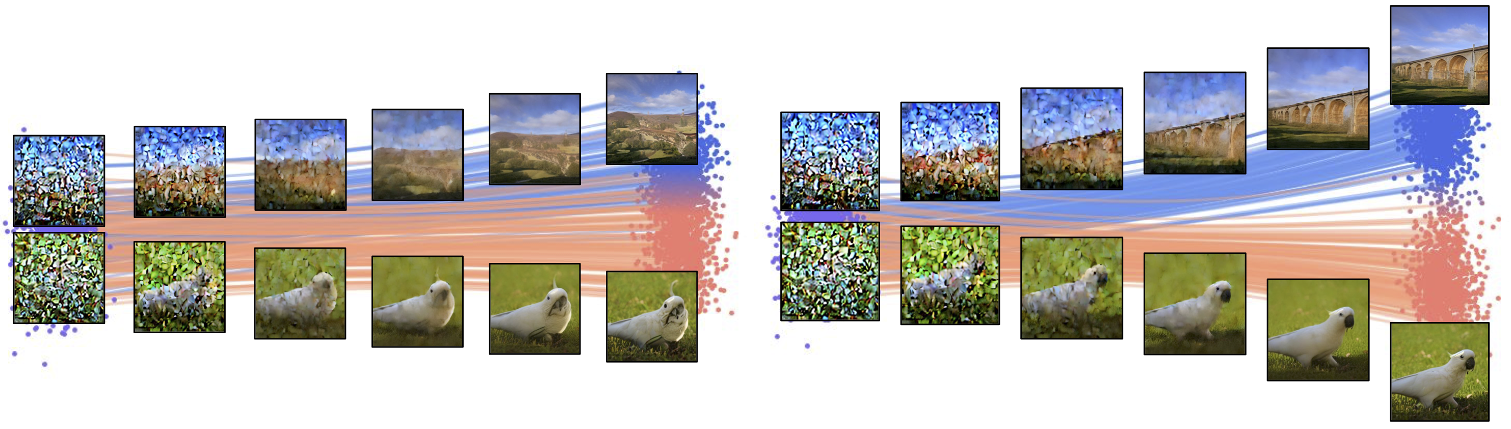
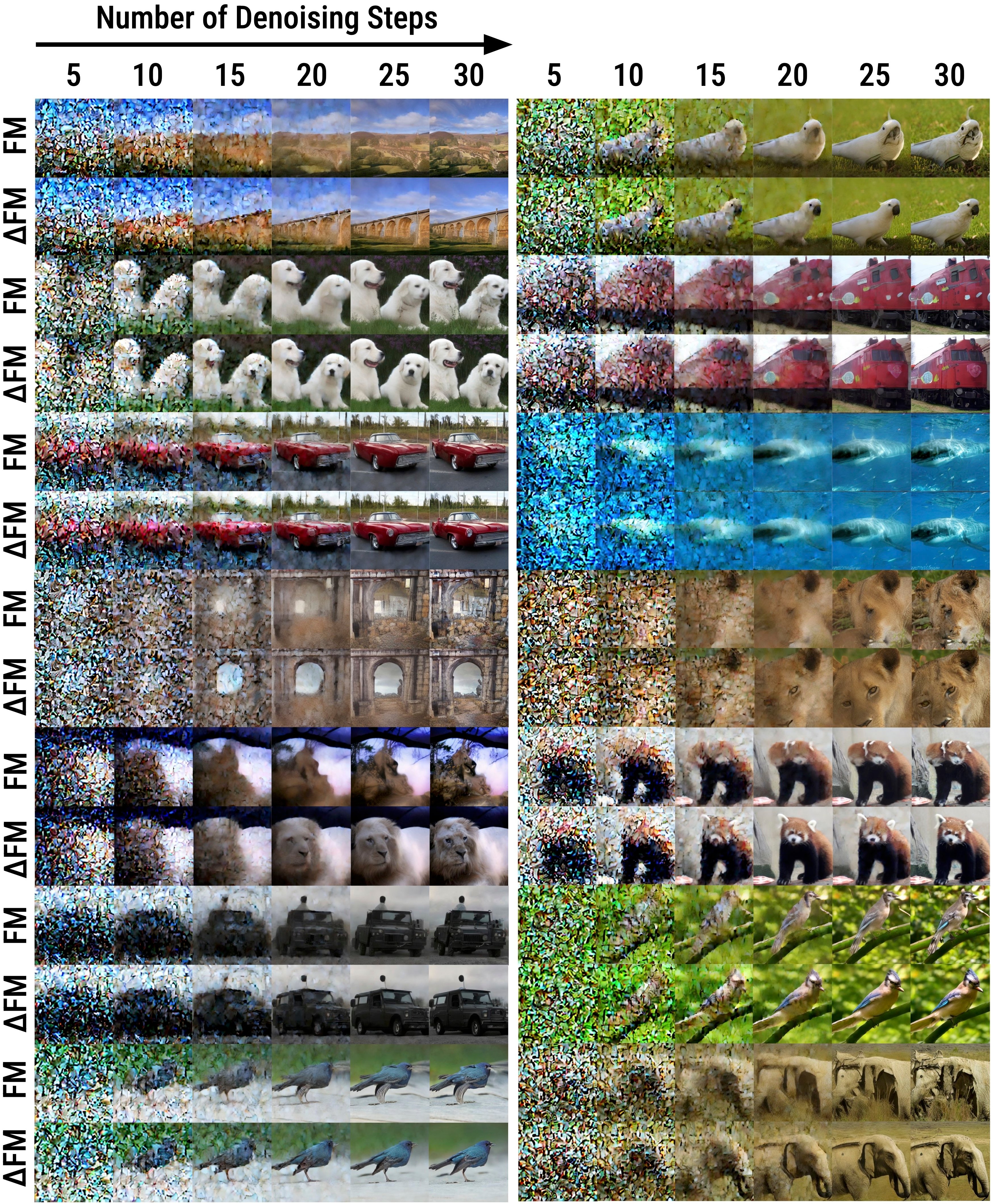
Earlier class differentiation during denoising. In Figure 4, we study flow trajectories of standard flow matching (FM) and flow matching with $\Delta$FM. To do this, we take partially denoised latents at various intermediate time steps along a trajectory with total length 30. While initially both follow similar trajectories, they quickly diverge within the first several steps of the denoising process. For instance, the model trained with $\Delta$FM produces more structurally coherent images earlier (around 15 to 20 steps in) than with FM. The iconic features of each class, such as slanted bridge surfaces (Figure 4 (top-left)), animal eyes (Figure 4 (upper-left and top-right), and train windows (Figure 4 (upper-right)), are more clearly visible early on during the diffusion process of the $\Delta$FM model. This enables $\Delta$FM to ultimately generate higher quality images at the final timestep.

		Metrics
Model	Batch Size	FID $\downarrow$	IS $\uparrow$	sFID $\downarrow$
REPA SiT-B/2	256	42.28	38.04	11.35
+ Using $\Delta$FM	256	33.39	43.44	05.67
REPA SiT-B/2	512	24.45	69.15	11.42
+ Using $\Delta$FM	512	17.06	81.41	05.29
REPA SiT-B/2	1024	22.00	76.15	11.76
+ Using $\Delta$FM	1024	15.23	88.53	05.20
REPA SiT-XL/2	256	11.14	115.83	8.25
+ Using $\Delta$FM	256	07.29	129.89	4.93
REPA SiT-XL/2	512	10.15	129.43	9.00
+ Using $\Delta$FM	512	06.36	146.17	5.42

Table 6: $\Delta$FM Scales with Batch Size. We train all models for 400K iterations and strictly follow the protocol of [44]. All metrics are measured with the SDE Euler-Maruyama sampler with NFE=50 and without classifier guidance. We use $\lambda=0.05$ for all models trained with $\Delta$FM and do not change any other hyperparameters. $\uparrow$ indicates that higher values are better, with $\downarrow$ denoting the opposite. Improvement using $\Delta$FM evenly scales with batch-size, and even outperforms flow-matching models with half the batch-size.

Effects of batch size on $\Delta$FM. In Table 6, we study the effects of batch size on our loss. It is well known that batch size has an important effect on contrastive style losses [5, 7, 15] that draw negatives within the batch. This can be understood as a sample diversity issue. If the batch size is larger than negative samples within the batch are more representative of the true distribution. In this table, we see a similar trend: larger batch sizes are important for maximizing the performance of $\Delta$FM across several model scales. We also maintain our improvements over the REPA baseline through all batch sizes and model scales.

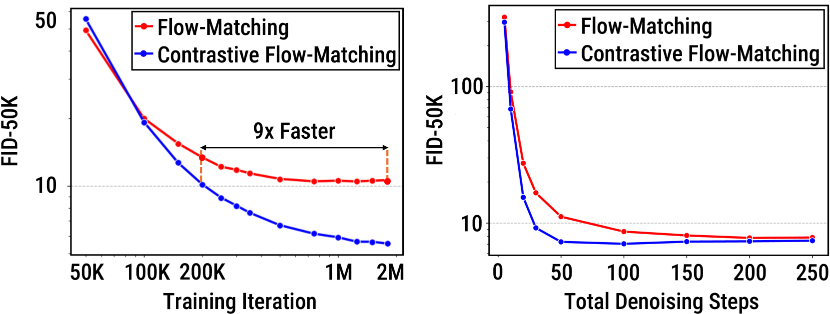
Improved training and inference speed. In Figure 5 (left), we see the significant improvements in training speed from the $\Delta$FM objective. We reach the same performance (measured by FID-50k) as baseline with $9\times$ fewer training iterations. In Figure 5 (right), we also demonstrate significant improvements at inference time. With our objective, we reach superior performance with only 50 denoising steps compared to the baseline with 250 denoising steps. This is a linear 5$\times$ improvement in training efficiency. Taken together, these results emphasize the important gains in computational efficiency achieved by our method.

Figure 5: $\Delta$FM requires significantly fewer training iterations and inference-time denoising steps. We plot FID-50k on ImageNet 256x256 with different numbers of training iterations and denoising steps. We see that $\Delta$FM outperforms the baseline with 9$\times$ fewer training iterations and 5$\times$ reduction in the number of inference-time denoising steps, indicating that $\Delta$FM is more efficient in both training and inference.

6 Conclusion

We introduced Contrastive Flow Matching ($\Delta$FM), a simple addition to the diffusion objective that enforces distinct, diverse flows during image generation. Quantitatively, $\Delta$FM results in improved image quality with far fewer denoising steps ($5\times$ faster) and significantly improved training speed ($9\times$ faster). Qualitatively, $\Delta$FM improves the structural coherence and global semantics for image generation. All of this is achieved with negligible extra compute per training iteration. Finally, we show that our improvements stack with the recently proposed Representation Alignment (REPA) loss, allowing for strong gains in image generation performance. Looking forward, $\Delta$FM shows the possibility that deviating from perfect distribution modeling in the diffusion objective might result in better image generation.

Figure 6: CC3M side-by-side generations between a REPA-MMDiT model trained with flow-matching (left) and $\Delta$FM (right). Models are trained for 400K iterations using a batch-size of 256 and images are generated without classifier-free guidance and using NFE=50.

Appendix A Text-to-Image Qualitative Results

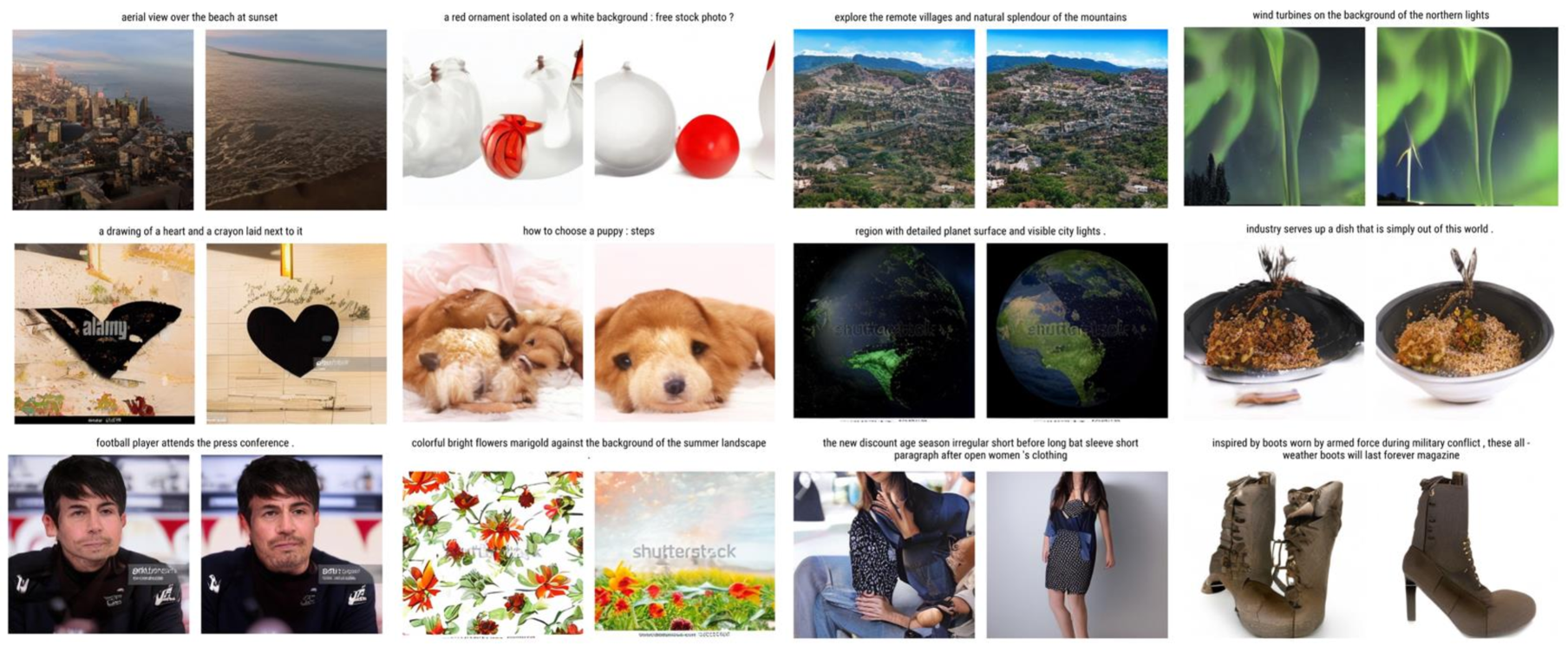
We visualize generations between our REPA-MMDiT models described in Section 5.3 trained with flow-matching (FM) loss and with $\Delta$FM on CC3M with a batch size of 256 for 400K iterations in Figure 6. We plot images in pairs, with FM images on the left and $\Delta$FM images on the right, and show the respective caption for each pair above. All images are generated without classifier-free guidance and using NFE=50, and are the same images used in Table 3.

Appendix B Deriving Contrastive-Flow Matching Interference

B.1 Closed-form solution to Eq. 4

We first re-introduce Eq. 4 for convenience,

$$\begin{split}\mathcal{L}^{(\textsc{$\Delta$FM})}(\theta)=\mathrm{E}\left[\begin{aligned} &||v_{\theta}(x_{t},t,y)-(\dot{\alpha}_{t}\hat{x}+\dot{\sigma}_{t}\epsilon)||^{2}\\ &-\lambda||v_{\theta}(x_{t},t,y)-(\dot{\alpha}_{t}\tilde{x}+\dot{\sigma}_{t}\tilde{\epsilon})||^{2}\end{aligned}\right]\end{split}$$

Minimizing the expectation, expanding all norms and letting $v(\theta)=v(x_{t},t,y)$, we can simplify the expectation to:

$$\begin{split}&=\min_{\theta}\mathrm{E}\left[\begin{aligned} (1-\lambda)v(\theta)^{T}v(\theta)\\ -2v(\theta)^{T}\left[(\dot{\alpha}_{t}\hat{x}+\dot{\sigma}_{t}\epsilon)-\lambda(\dot{\alpha}_{t}\tilde{x}+\dot{\sigma}_{t}\tilde{\epsilon})\right]\\ +(\dot{\alpha}_{t}\hat{x}+\dot{\sigma}_{t}\epsilon)^{T}(\dot{\alpha}_{t}\hat{x}+\dot{\sigma}_{t}\epsilon)\\ -\lambda(\dot{\alpha}_{t}\tilde{x}+\dot{\sigma}_{t}\tilde{\epsilon})^{T}(\dot{\alpha}_{t}\tilde{x}+\dot{\sigma}_{t}\tilde{\epsilon})\end{aligned}\right]\end{split}$$ (7)

$$\begin{split}&=\min_{\theta}\mathrm{E}\left[\begin{aligned} (1-\lambda)v(\theta)^{T}v(\theta)\\ -2v(\theta)^{T}\left[(\dot{\alpha}_{t}\hat{x}+\dot{\sigma}_{t}\epsilon)-\lambda(\dot{\alpha}_{t}\tilde{x}+\dot{\sigma}_{t}\tilde{\epsilon})\right]\end{aligned}\right]\end{split}$$ (8)

$$\begin{split}&\mathrel{\vbox{ \offinterlineskip\halign{\hfil$#$\cr\propto\cr\kern 2.0pt\cr\sim\cr\kern-2.0pt\cr}}}\min_{\theta}\mathrm{E}\left[\left|\left|\begin{aligned} \sqrt{1-\lambda}v(\theta)\\ -\frac{(\dot{\alpha}_{t}\hat{x}+\dot{\sigma}_{t}\epsilon)-\lambda(\dot{\alpha}_{t}\tilde{x}+\dot{\sigma}_{t}\tilde{\epsilon})}{\sqrt{1-\lambda}}\end{aligned}\right|\right|^{2}_{2}\right]\end{split}$$ (9)

Setting the gradient with respect to $v(\theta)$ to $0$,

$$\sqrt{1-\lambda}v(\theta)^{*} =\mathrm{E}\left[\frac{(\dot{\alpha}_{t}\hat{x}+\dot{\sigma}_{t}\epsilon)-\lambda(\dot{\alpha}_{t}\tilde{x}+\dot{\sigma}_{t}\tilde{\epsilon})}{\sqrt{1-\lambda}}\right]$$ (10)

$$v(\theta)^{*} =\frac{\mathrm{E}\left[\dot{\alpha}_{t}\hat{x}+\dot{\sigma}_{t}\epsilon\right]-\lambda\mathrm{E}\left[\dot{\alpha}_{t}\tilde{x}+\dot{\sigma}_{t}\tilde{\epsilon}\right]}{1-\lambda}$$ (11)

Finally, observe that $\mathrm{E}\left[\dot{\alpha}_{t}\hat{x}+\dot{\sigma}_{t}\epsilon\right]$ is the solution to the flow-matching objective. Setting $\mathrm{E}\left[\dot{\alpha}_{t}\tilde{x}+\dot{\sigma}_{t}\tilde{\epsilon}\right]=\hat{T}$ and observing that $x_{t}$ does not depend on $\hat{x}$ or $\hat{\epsilon}$ we obtain:

$$\min_{\theta}\mathcal{L}^{(\Delta\text{FM})}(\theta)=\frac{\min_{\theta}\mathcal{L}^{(\text{FM})}(\theta)-\lambda\hat{T}}{1-\lambda}$$ (12)

B.2 Coupling with CFG

Classifier-free guidance (CFG) is originally defined over the flow-matching solution of $\min_{\theta}\mathcal{L}^{(\text{FM})}$. Re-writing Eq. 12 and substituting it into the CFG equation, we obtain:

$$CFG=wv^{(FM)}(x_{t},t,y)+(1-w)v^{(FM)}(x_{t},t,\emptyset)$$ (13)

$$\begin{split}&=\left[\begin{aligned} w\left[(1-\lambda)v^{(\textsc{$\Delta$FM})}(x_{t},t,y)+\lambda\hat{T}\right]\\ -(1-w)\left[(1-\lambda)v^{(\textsc{$\Delta$FM})}(x_{t},t,\emptyset)+\lambda\hat{T}\right]\end{aligned}\right]\end{split}$$ (14)

$$\begin{split}&=\left[\begin{aligned} (1-\lambda)\left[\begin{aligned} wv^{(\textsc{$\Delta$FM})}(x_{t},t,y)\\ +(1-w)v^{(\textsc{$\Delta$FM})}(x_{t},t,\emptyset)\end{aligned}\right]\end{aligned}+\lambda\hat{T}\right]\end{split}$$ (15)

Letting $v(x_{t}|y)=v^{(\textsc{$\Delta$FM})}(x_{t},t,y)$ and $v(x_{t}|\emptyset)=v^{(\textsc{$\Delta$FM})}(x_{t},t,\emptyset)$, we obtain the Eq. from Section 5.4: $\hat{CFG}=(1-\lambda)\left[wv(x_{t}|y)+(1-w)v(x_{t}|\emptyset)\right]+\lambda\hat{T}$.

References

- Albergo and Vanden-Eijnden [2022] Michael S Albergo and Eric Vanden-Eijnden. Building normalizing flows with stochastic interpolants. arXiv preprint arXiv:2209.15571, 2022.
- Albergo et al. [2023] Michael S Albergo, Nicholas M Boffi, and Eric Vanden-Eijnden. Stochastic interpolants: A unifying framework for flows and diffusions. arXiv preprint arXiv:2303.08797, 2023.
- Bao et al. [2023] Fan Bao, Shen Nie, Kaiwen Xue, Yue Cao, Chongxuan Li, Hang Su, and Jun Zhu. All are worth words: A vit backbone for diffusion models. In CVPR, 2023.
- Cao et al. [2017] Gongze Cao, Yezhou Yang, Jie Lei, Cheng Jin, Yang Liu, and Mingli Song. Tripletgan: Training generative model with triplet loss, 2017.
- Caron et al. [2021] Mathilde Caron, Hugo Touvron, Ishan Misra, Hervé Jégou, Julien Mairal, Piotr Bojanowski, and Armand Joulin. Emerging properties in self-supervised vision transformers. In ICCV, 2021.
- Chen et al. [2018] Ricky T. Q. Chen, Yulia Rubanova, Jesse Bettencourt, and David Duvenaud. Neural ordinary differential equations. In Advances in Neural Information Processing Systems, 2018.
- Chen et al. [2020] Ting Chen, Simon Kornblith, Mohammad Norouzi, and Geoffrey Hinton. A simple framework for contrastive learning of visual representations. ICLR, 2020.
- Chung et al. [2022] Hyungjin Chung, Jeongsol Kim, Michael T Mccann, Marc L Klasky, and Jong Chul Ye. Diffusion posterior sampling for general noisy inverse problems. arXiv preprint arXiv:2209.14687, 2022.
- Chung et al. [2024] Hyungjin Chung, Jeongsol Kim, Geon Yeong Park, Hyelin Nam, and Jong Chul Ye. Cfg++: Manifold-constrained classifier free guidance for diffusion models. arXiv preprint arXiv:2406.08070, 2024.
- Deng et al. [2009] Jia Deng, Wei Dong, Richard Socher, Li-Jia Li, Kai Li, and Li Fei-Fei. Imagenet: A large-scale hierarchical image database. In 2009 IEEE conference on computer vision and pattern recognition, pages 248–255. Ieee, 2009.
- Desai and Vasconcelos [2024] Alakh Desai and Nuno Vasconcelos. Improving image synthesis with diffusion-negative sampling, 2024.
- Dhariwal and Nichol [2021] Prafulla Dhariwal and Alexander Nichol. Diffusion models beat gans on image synthesis. Advances in neural information processing systems, 34:8780–8794, 2021.
- Dosovitskiy et al. [2021] Alexey Dosovitskiy, Lucas Beyer, Alexander Kolesnikov, Dirk Weissenborn, Xiaohua Zhai, Thomas Unterthiner, Mostafa Dehghani, Matthias Minderer, Georg Heigold, Sylvain Gelly, Jakob Uszkoreit, and Neil Houlsby. An image is worth 16x16 words: Transformers for image recognition at scale. In ICLR, 2021.
- Esser et al. [2024] Patrick Esser, Sumith Kulal, Andreas Blattmann, Rahim Entezari, Jonas Müller, Harry Saini, Yam Levi, Dominik Lorenz, Axel Sauer, Frederic Boesel, Dustin Podell, Tim Dockhorn, Zion English, and Robin Rombach. Scaling rectified flow transformers for high-resolution image synthesis. ICML, 2024.
- He et al. [2020] Kaiming He, Haoqi Fan, Yuxin Wu, Saining Xie, and Ross Girshick. Momentum contrast for unsupervised visual representation learning. CVPR, 2020.
- Heusel et al. [2017] Martin Heusel, Hubert Ramsauer, Thomas Unterthiner, Bernhard Nessler, and Sepp Hochreiter. Gans trained by a two time-scale update rule converge to a local nash equilibrium. Advances in neural information processing systems, 30, 2017.
- Ho and Salimans [2022a] Jonathan Ho and Tim Salimans. Classifier-free diffusion guidance. arXiv preprint arXiv:2207.12598, 2022a.
- Ho and Salimans [2022b] Jonathan Ho and Tim Salimans. Classifier-free diffusion guidance, 2022b.
- Ho et al. [2020] Jonathan Ho, Ajay Jain, and Pieter Abbeel. Denoising diffusion probabilistic models. In Advances in Neural Information Processing Systems, 2020.
- Karras et al. [2024] Tero Karras, Miika Aittala, Tuomas Kynkäänniemi, Jaakko Lehtinen, Timo Aila, and Samuli Laine. Guiding a diffusion model with a bad version of itself. arXiv preprint arXiv:2406.02507, 2024.
- [21] Felix Koulischer, Johannes Deleu, Gabriel Raya, Thomas Demeester, and Luca Ambrogioni. Dynamic negative guidance of diffusion models: Towards immediate content removal. In Neurips Safe Generative AI Workshop 2024.
- Kynkäänniemi et al. [2019] Tuomas Kynkäänniemi, Tero Karras, Samuli Laine, Jaakko Lehtinen, and Timo Aila. Improved precision and recall metric for assessing generative models. NeurIPS, 2019.
- Kynkäänniemi et al. [2024] Tuomas Kynkäänniemi, Miika Aittala, Tero Karras, Samuli Laine, Timo Aila, and Jaakko Lehtinen. Applying guidance in a limited interval improves sample and distribution quality in diffusion models. arXiv preprint arXiv:2404.07724, 2024.
- Lipman et al. [2023a] Yaron Lipman, Ricky T. Q. Chen, Heli Ben-Hamu, Maximilian Nickel, and Matthew Le. Flow matching for generative modeling. In ICLR, 2023a.
- Lipman et al. [2023b] Yaron Lipman, Ricky T. Q. Chen, Heli Ben-Hamu, Maximilian Nickel, and Matthew Le. Flow matching for generative modeling. In ICLR, 2023b.
- Liu et al. [2022] Xingchao Liu, Chengyue Gong, and Qiang Liu. Flow straight and fast: Learning to generate and transfer data with rectified flow, 2022.
- Lu et al. [2023] Cheng Lu, Huayu Chen, Jianfei Chen, Hang Su, Chongxuan Li, and Jun Zhu. Contrastive energy prediction for exact energy-guided diffusion sampling in offline reinforcement learning. In International Conference on Machine Learning, pages 22825–22855. PMLR, 2023.
- Luo et al. [2023] Simian Luo, Yiqin Tan, Longbo Huang, Jian Li, and Hang Zhao. Latent consistency models: Synthesizing high-resolution images with few-step inference. arXiv preprint arXiv:2310.04378, 2023.
- Ma et al. [2024] Nanye Ma, Mark Goldstein, Michael S. Albergo, Nicholas M. Boffi, Eric Vanden-Eijnden, and Saining Xie. Sit: Exploring flow and diffusion-based generative models with scalable interpolant transformers. 2024.
- Nash et al. [2021] Charlie Nash, Jacob Menick, Sander Dieleman, and Peter W Battaglia. Generating images with sparse representations. arXiv preprint arXiv:2103.03841, 2021.
- Oquab et al. [2024] Maxime Oquab, Timothée Darcet, Théo Moutakanni, Huy V. Vo, Marc Szafraniec, Vasil Khalidov, Pierre Fernandez, Daniel HAZIZA, Francisco Massa, Alaaeldin El-Nouby, Mido Assran, Nicolas Ballas, Wojciech Galuba, Russell Howes, Po-Yao Huang, Shang-Wen Li, Ishan Misra, Michael Rabbat, Vasu Sharma, Gabriel Synnaeve, Hu Xu, Herve Jegou, Julien Mairal, Patrick Labatut, Armand Joulin, and Piotr Bojanowski. DINOv2: Learning robust visual features without supervision. TMLR, 2024.
- Rombach et al. [2022] Robin Rombach, Andreas Blattmann, Dominik Lorenz, Patrick Esser, and Björn Ommer. High-resolution image synthesis with latent diffusion models. In Proceedings of the IEEE/CVF conference on computer vision and pattern recognition, pages 10684–10695, 2022.
- Russakovsky et al. [2015] Olga Russakovsky, Jia Deng, Hao Su, Jonathan Krause, Sanjeev Satheesh, Sean Ma, Zhiheng Huang, Andrej Karpathy, Aditya Khosla, Michael Bernstein, Alexander C. Berg, and Li Fei-Fei. Imagenet large scale visual recognition challenge, 2015.
- Salimans and Ho [2022] Tim Salimans and Jonathan Ho. Progressive distillation for fast sampling of diffusion models. arXiv preprint arXiv:2202.00512, 2022.
- Salimans et al. [2016] Tim Salimans, Ian Goodfellow, Wojciech Zaremba, Vicki Cheung, Alec Radford, and Xi Chen. Improved techniques for training gans. Advances in neural information processing systems, 29, 2016.
- Schroff et al. [2015] Florian Schroff, Dmitry Kalenichenko, and James Philbin. Facenet: A unified embedding for face recognition and clustering. In 2015 IEEE Conference on Computer Vision and Pattern Recognition (CVPR), page 815–823. IEEE, 2015.
- Sharma et al. [2018] Piyush Sharma, Nan Ding, Sebastian Goodman, and Radu Soricut. Conceptual captions: A cleaned, hypernymed, image alt-text dataset for automatic image captioning. In Proceedings of ACL, 2018.
- Shenoy et al. [2024] Rahul Shenoy, Zhihong Pan, Kaushik Balakrishnan, Qisen Cheng, Yongmoon Jeon, Heejune Yang, and Jaewon Kim. Gradient-free classifier guidance for diffusion model sampling. arXiv preprint arXiv:2411.15393, 2024.
- Song et al. [2021] Jiaming Song, Chenlin Meng, and Stefano Ermon. Denoising diffusion implicit models. In International Conference on Learning Representations, 2021.
- Song et al. [2023] Jiaming Song, Qinsheng Zhang, Hongxu Yin, Morteza Mardani, Ming-Yu Liu, Jan Kautz, Yongxin Chen, and Arash Vahdat. Loss-guided diffusion models for plug-and-play controllable generation. In International Conference on Machine Learning, pages 32483–32498. PMLR, 2023.
- Vahdat et al. [2021] Arash Vahdat, Karsten Kreis, and Jan Kautz. Score-based generative modeling in latent space, 2021.
- Yin et al. [2024a] Tianwei Yin, Michaël Gharbi, Taesung Park, Richard Zhang, Eli Shechtman, Fredo Durand, and William T Freeman. Improved distribution matching distillation for fast image synthesis. arXiv preprint arXiv:2405.14867, 2024a.
- Yin et al. [2024b] Tianwei Yin, Michaël Gharbi, Richard Zhang, Eli Shechtman, Fredo Durand, William T Freeman, and Taesung Park. One-step diffusion with distribution matching distillation. In Proceedings of the IEEE/CVF Conference on Computer Vision and Pattern Recognition, pages 6613–6623, 2024b.
- Yu et al. [2024] Sihyun Yu, Sangkyung Kwak, Huiwon Jang, Jongheon Jeong, Jonathan Huang, Jinwoo Shin, and Saining Xie. Representation alignment for generation: Training diffusion transformers is easier than you think, 2024.
- Zhao et al. [2022] Min Zhao, Fan Bao, Chongxuan Li, and Jun Zhu. Egsde: Unpaired image-to-image translation via energy-guided stochastic differential equations. Advances in Neural Information Processing Systems, 35:3609–3623, 2022.
- Zhou et al. [2024] Mingyuan Zhou, Zhendong Wang, Huangjie Zheng, and Hai Huang. Long and short guidance in score identity distillation for one-step text-to-image generation. arXiv preprint arXiv:2406.01561, 2024.